Using WideBand Example Tracings on the GSI TympStar Pro
There are a lot of reasons to be excited about incorporating WideBand Tympanometry into daily clinical practice when analyzing the middle ear system. From a practical perspective, it couldn’t be easier to perform a WideBand Tympanometry test. It is the exact same procedure as taking traditional tympanometry measurements and takes the same amount of time. However, what is not so straightforward is how we interpret and report the results. One simple way to start is by comparing obtained WideBand results against pre-loaded example tracings.
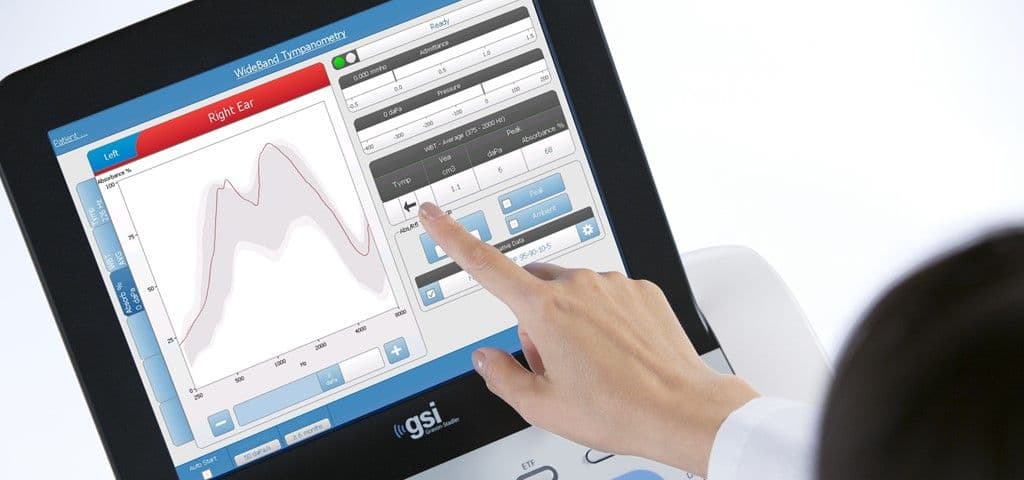
The example tracings can be accessed from the Absorbance tab, which is the third of three tabs that are generated with every WideBand sweep. After the test is complete the first tab populates with four single frequency tympanograms.
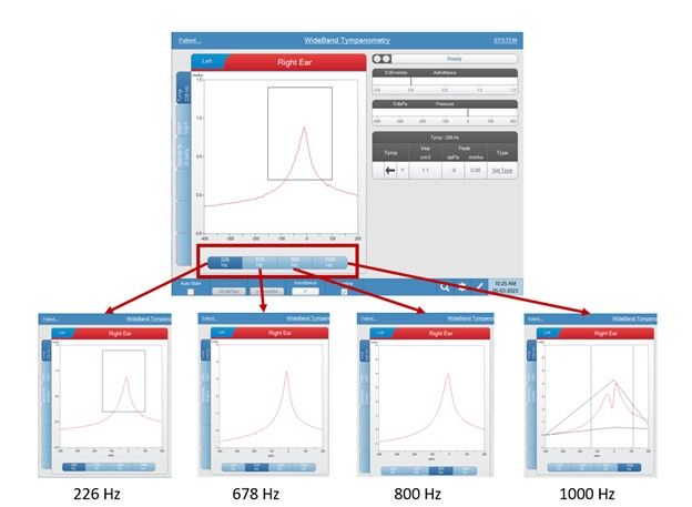
Scrolling through the four single frequency tymps should be the first step in interpretation. Interpreting these results within the constellation of audiometric findings is something we are very familiar with and provides us the initial framework with which to view the WideBand Average Tymp (WBT) and Absorbance tabs.
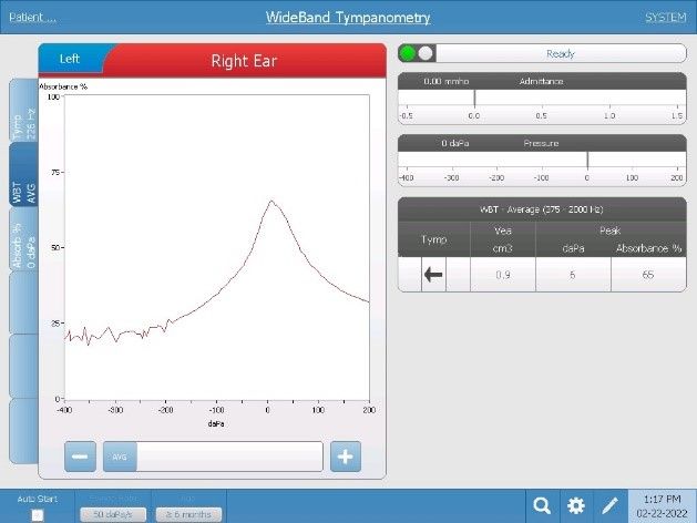
The WideBand Average Tymp tab gives us the average of all the single frequency in range that is based on age. For adults, this average is 375-2000 Hz and for infants under 6 months, 800-2000 Hz. While this WideBand tympanogram appears similar in morphology to a single frequency tympanogram, it is important to keep a few things in mind. First off, we are viewing the pressure sweep as a function of the percentage of absorbance, rather than admittance we are used to viewing with traditional tympanometry. One advantage of averaging is that it can be helpful if there was movement or noise during testing.
Example of noise during the test:
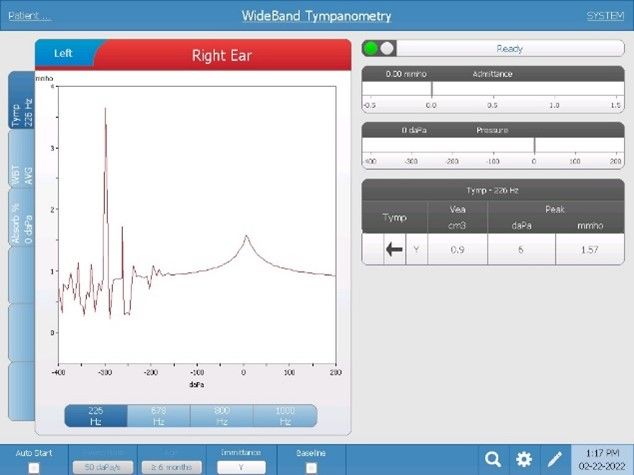
The WideBand Average Tymp for the same test:
While there are differences between the tympanometry types in Tab 1 and the WBT in Tab 2, the deep familiarity we already have with traditional tymps sets us up quickly develop a sense of what is happening with the WBT. It isn’t until we get to Tab 3 and the Absorbance graph where we are plotting out the percentage of absorbance as a function of frequency. The WideBand click stimulus is comprised of acoustic energy between 250 and 800 Hz, and the absorbance curve is showing us how sound is being absorbed as a function of pressure. Interpreting the absorbance graphs may not be as immediately familiar in the way that a WBT is somewhat similar to single frequency tympanometry. That is where the example tracings can come in handy.
Let first take a look at typical absorbance curve that you might see with someone who has a classic type A tympanogram measure at 226 Hz.
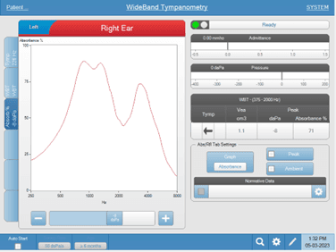
In addition to the curve showing us the response at Tympanic Peak Pressure (TPP), we can see an estimated ECV, TPP, and overall percentage of absorbance. To view normative data and the included example tracings, select the gear icon in the Absorbance/Reflectance Settings.
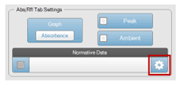
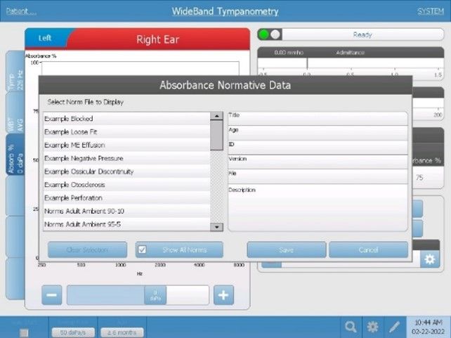
That will open a dialog box with the example tracings at the top of the list:
Let’s go through them one by one and point out some of the key characteristics associated with each condition. In the examples below we will see a typical WideBand tracing, which is the bold red or blue line on the absorbance graph. The Example tracing is more subtle dotted line superimposed on the graph.
The first two we will look at are less about identifying pathology and more about the integrity of the overall test. If our probe is blocked due to debris in the eartip, or if the probe was pressed against the canal wall/debris in the canal there is a fairly typical tracing which has extremely low absorbance across all frequencies.

The second example is what we are likely to see if we have a loose fitting probe or shallow insertion of the probe in the canal during testing. These are characterized by very high absorbance in the low frequencies with lots of variability in peaks and valleys across the entire range.
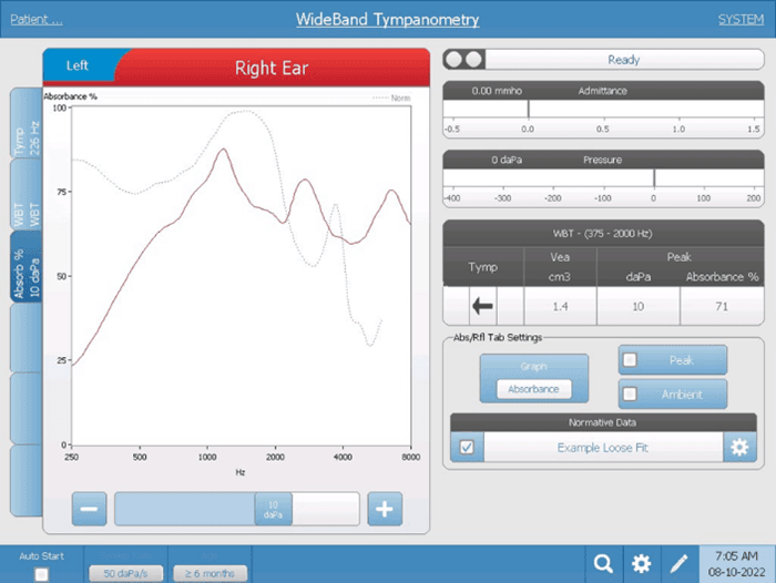
A good way of determining if the probe fit is contributing to excessive low frequency absorbance is by looking at where absorbance is at 250 Hz. Anything above about 25% (as indicated by the red arrow above) should be suspect, and a new sweep is suggested.
Now let’s look at some common pathologies and what we might expect to see in the absorbance tab. If our 226 Hz tymp from tab 1 is consistent with a type C or type B tympanogram tracing with age appropriate ECV’s, we are likely to see a tracing that shows low absorbance in the low frequencies when viewed at Ambient Pressure (0 daPa).
In this example, we see the typical pattern for negative pressure plotted against an absorbance graph at ambient pressure for someone with a TPP of -273 with a classic type C tympanogram.
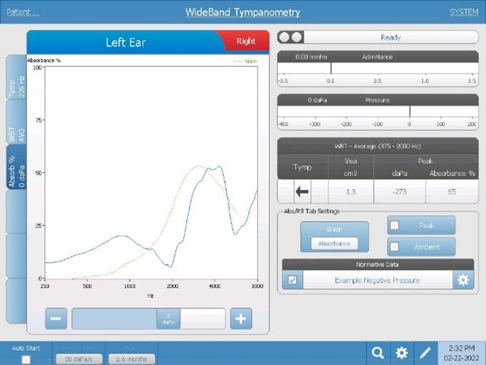
With Negative pressure we are also likely to see the absorbance showing a relatively normal pattern when viewed at TPP. In this example, we see excessive negative pressure (-367 daPa). The blue line showing us absorbance at that peak and the purple line showing us absorbance at ambient pressure.
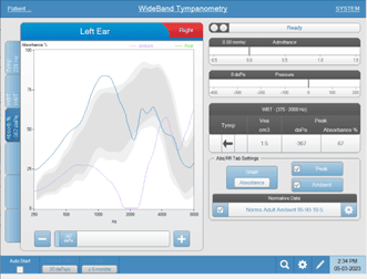
In this example, we also see normative data superimposed for ambient pressure, and we can see how the tracing at peak follows along with this pattern.
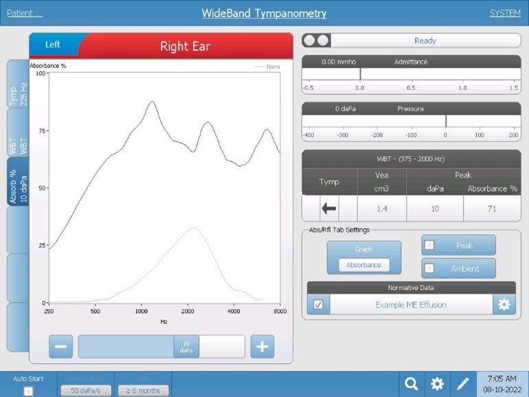
When we progress beyond negative pressure and get into middle ear effusion we see a similar pattern as with negative pressure with less overall absorbance and an additional reduction in higher frequencies.
A tympanic membrane with a perforation will have variability depending on the size of the perforation. We often see increased absorbance below 2k, with some smaller perforations may show peak around 1k. Peaks tend to shift to higher frequencies with larger perforations, with very large perforations showing normal absorbance in LF and very high in HFs.

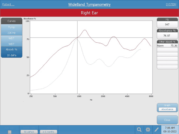
In cases of suspected ossicular discontinuity there tends to be a pronounced absorbance peak around 700-900 Hz. Using the zoom feature (magnifying glass icon) on the TympStar Pro allows us to determine very easily where the absorbance tracing is peaking in these instances.
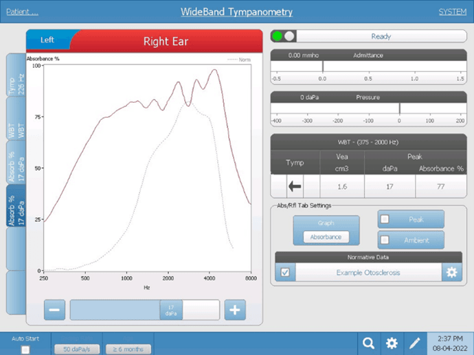
In our final example we see a tracing consistent with Otosclerosis. This condition is characterized by reduced absorbance in lower frequencies (1-2 kHz). As stiffness increases, absorbance decreases in low frequencies, with high frequencies less affected.
Visit the linked page for more information about using WideBand Tympanometry.
Tony received his master’s from the University of Wisconsin-Oshkosh with an emphasis on pediatric audiology. He has over 20 years of experience in the hearing industry and has worked in a variety of settings. He has experience performing diagnostic testing with all age ranges, industrial audiology, retail, hearing aid financing and insurance, practice development programs and industry trade shows. At GSI, Tony is focused on training, support and education.